A Rhythm Map is a heat map that displays time in the X and Y dimensions. They are an excellent way to visualize repeating patterns in time, such as how crimes occur by hour and data of week. Here we look at some interesting patterns in burglaries in the City of San Diego. First, here is the map for a range of crime types in San Diego, compiled from the type, time and date of about 400K crime incidents in the City of San Diego from 2006 to 2012.   Each square is a crime type. The vertical axis is the hour of the day, and the horizontal axis is the day of the week, with Sunday being the cell between 0 and 1. Darker red means there are more crimes than lighter red and yellow. The colors are not comparable across squares, only within the cell. So, the dark red cell at 5:00PM on Friday in the Burglary square may represent a very different number of crime incidents than then dark red cell at 12:00AM on Thursday in Sex Crimes. Also note that these views combine citations, arrests and reported crimes, and there may be different patters when the maps are broken out on that factor. There are a lot of interesting patterns here, but we’ll focus on Burglary. The first thing to notice is there are two time ranges, groups of darker red cells, when burglaries occur: during the work hours on weekdays and on Friday evenings. ( The strong line at noon is most likely an artifact of crimes for which the time is not known being given that value arbitrarily. ) What accounts for the two separate time ranges? First, let’s break it out by community. This chart uses Clarinova Place Codes for the community names.   Here we see that some communities exhibit one pattern or the other, and sometimes both. Downtown ( SanDOW ), La Jolla ( SanLAJ ) and Mira Mesa ( SanMIR ) show the Friday pattern, while Southeastern ( SanSOT), Greater North Park ( SanGRE) and Midtown ( SanMID ) show the week day pattern. Community distinctions may explain some of the differences in the patterns, but there is a factor that is probably more important: residential vs commercial crime. So, let’s split out the maps on that factor. Here is where the distinctions become the strongest. In Otay Mesa ( SanOAT ), Mira Mesa ( SanMIR ) University ( SanUNV ) and others, the Friday evening pattern completely splits from the weekday pattern. However, we also see a new weekday pattern in the commercial burglaries in Claremont ( SanCLA ), Uptown, Midtown, with commercial burglaries occurring across the weekday evenings. Those features are consistent with exactly what you’d expect from burglary: the burglaries occur when the business and homes are unoccupied. But it doesn’t explain why in many communities the commercial crimes would occur more frequently on Friday evenings. Another unusual pattern is that in Pacific Beach ( SanPCF ) there is a residential burglary cluster on Friday and Saturday evenings, with a similar but weaker pattern occurring in Uptown and College. Rhythms are a powerful way to look for patterns in time-structured data, because they take advantage of the ways that human brains most quickly process visual information. However, they aren’t a complete solution; they are just a start. Before making any recommendations based on the data, we’d want to do a few statistical tests, and at least, look at the absolute number of incidents per cell in the areas exhibiting patterns.

Here is an interactive data application that explores how crime incidents vary over the day of week and time of day. In the checkbox below, select one or more crime types, and the heatmap will show the relative intensity of those crime types over day of week and time of day. There many interesting patterns here, some you would expect, some you might not: Things you might expect:

• DUI and Drugs violations are primarily committed in the evening and early mornings on weekends.
• Assaults are most frequent in the late evenings and early mornings on weekends.
• Vehicle theft and break-ins are committed in the dark.
• Burglary is committed during the day, while people are at work.

There are also a few interesting surprises:

We recently converted the SWITRS database of traffic collisions in California, extracting the records for San Diego County and creating a basic visualization in Tableau Public. Tableau Public is a fantastic data analysis tool, although it takes a bit of training to do complex things. Below is a simple visualization of the number of people killed and injured in San Diego county traffic collisions by day of week and hour of day, for the years 2002 to 2012, inclusive. The deaths line (orange) shows a familiar “bathtub” shape, with higher values on weekends and at night. The injured line is quite different. There are a lot of possibilities for this, including statistical effects due to the 100x difference in the number of injuries and deaths, or the qualitative differences between pedestrians at night during those of the day. For instance, it may be that injuries during the day are driven by travel patterns and reduced attentiveness in the afternoon, while fatalities are driven by alcohol consumption. Fortunately, there is enough information in the SWITRS dataset to test some of these hypothesis, but that will be the subject of another post.

A few weeks ago, we received crime incident data from SANDAG for the years from 2007 to March of 2013. The data has the location of the crime listed as a “hundred block,” so a crime at 1435 Main street would be listed at 1400 Main. Since we don’t know where the crime occurred on the block - we don’t know the exact address - it makes sense to attribute the crime to the whole block. I just finished an initial pass at geocoding crimes to street segments, using the All_Roads file from SANGIS and lot of custom Python code. Here are the results: 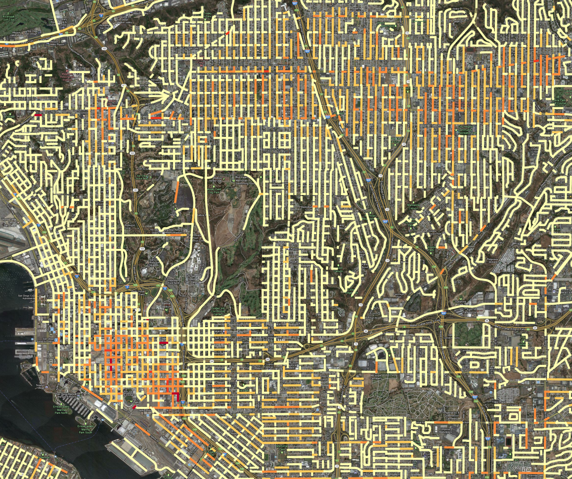All crime incidents for 2007 to 2013, colored according to linear density on the street segment. In this map, all of the crime incidents for the 6 year period are counted, grouped by the block where the crime occurred. Then, the counts are divided by the length of the street segment and the time period, so the final value is Crime per year per kilometer. Then, the range of values is broken into 5 groups, using the Jenks natural breaks. ( Using head/tail breaks would require more programming ) I tweaked the breaks manually to put more segments into the top category. This presentation has an advantage over the previous maps we’d created, using Kernel Density Estimation to produce heatmaps: it is easier to see where high-crime blocks are. For instance, lets look at the red block east of downtown, due south of Balboa park. A crack house, perhaps? 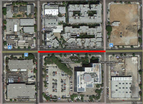Nope, it is the Police station. It is very common for crimes to have their address set to the police station if it isn’t clear what an appropriate address would be, such as for a car chase or someone caught in a canyon, like in this hotspot in Mission Gorge: 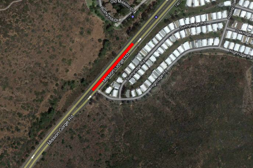  It isn’t likely that the particular segment of road gets a lot of crimes, and the criminals probably don’t live in the mobile home park. That segment of road probably contains the address number that is used for crime committed in Mission Gorge, it maybe it is where the cops like to park to patrol the canyon. Here is a real hotspot, an empty lot that seems to be popular for drug use: 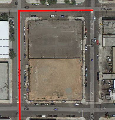Compare this to the heatmap view, zoomed out to show the contour of the hotspot: 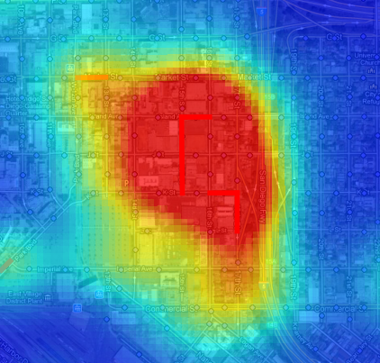The heatmap works better at small scales, because you can quickly assess an entire region. At large scales, the street segment view can help isolate what a likely cause of the problem is, which can obscured by the large regions of the heatmap hotspots. The heat map also encourages a subtle psychological bias: the larger areas seem more significant, because our brains place a lot of emphasis on size. But in the segment map, the segments are viewed discretely, as qualities, not extents. So, it is easier to pay attention to unusual high intensity blocks which pop up because they are bright red, but which in the heatmap get ignored because they are small. We’re not quite ready to publish the processed crime data, but should have it released, along with both kinds of maps, in the next week.

SANDAG Senior Research Analyst Mike Calandra sent us some traffic data updates for our Data As a Public Good report. I’m always thrilled when I get to communicate directly with agency analysts, and having them write to me is like an early Christmas. In our Data as a Public Good report several interviewees reported that they had difficulty getting traffic data from SANDAG, and the SANDAG website only publishes traffic count data as a PDF or an interactive map. However, SANDAG was very responsive to my Public Records Act Request for the traffic counts in a structured format, and we’ve got the response from that request in our repository, so we’ve updated the report to reflect this more recent experience, and here are some other resources that Mike mentioned. SANDAG is current in the process of updating their traffic count reports and replacing them with a Regional Count Database. The application will be an interactive map with a focus on arterial streets. CalTRANS, through their PEMS application, reports counts for freeways. PEMS also has about 10 years of data for many other traffic metrics, such as collisions. Every 10 years, SANDAG does a survey of county residents about travel. The last one was conducted in 2006. I haven’t read the report in enough detail to assess the quality of the statistics, but I’m already really impressed with the design and methodology – see “Cognitive Interview” appendix on page 132 for a lesson on how to do a survey right. If the survey company, NUSTATS, put as much work into statistics that they did in designing the survey, this report has the best data it would be possible to get. Mike sent a few other links that I knew existed, but hadn’t seen, such as these links to forecasts:

Here is some eye candy, a population density map of Pacific Beach and surrounding neighborhoods.

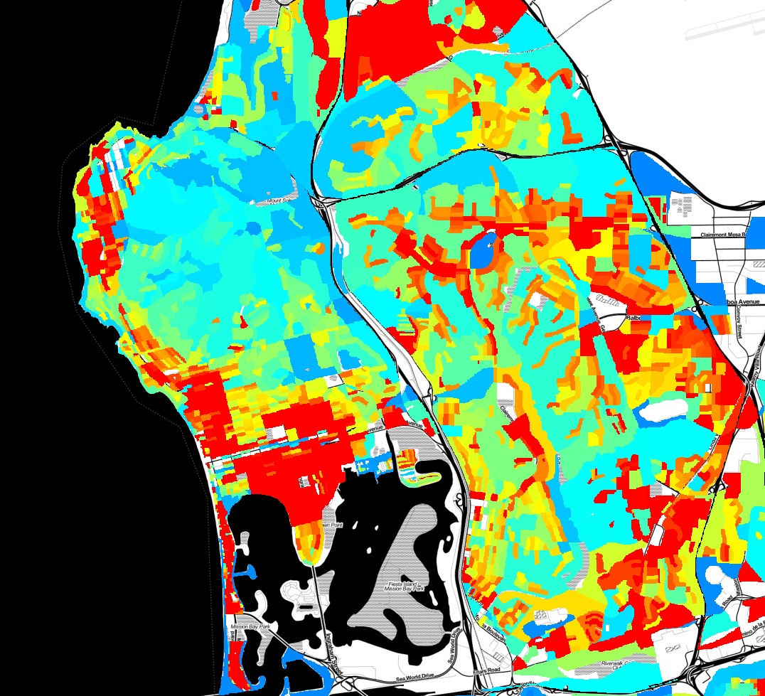
This map was created with a lot of Python code, using the 2010 census shapefiles for census blocks, setting a value for each block as the population of the block divided by the area of the block, and rasterizing all of the blocks to an image. Red indicates areas of higher population density. You can clearly pick out the areas in Pacific Beach that are zoned for apartments vs single family homes, the UTC high-rise apartment area, and many other variations in land use.

I’m spending the morning at Qualcomm for the Python Data Analysis Workshop, run by Dave Cook of the San Diego Python User group. I’m presenting about using Python to analyze crime and census data. If you like pretty pictures, the presentation has plenty of them:

Analyzing Crime and Census Data Presentation.

We’ve released a new report, Municipal Open Data Policies. The best way to ensure that San Diego area nonprofits and citizens get useful data is for local governments to adopt Open Data policies. These policies, which have been implemented in many cities around the country, mandate that cities publish data. So, instead of fighting for months to get data through a Public Records Act request, you can just download what you want from a website. Our latest report, Municipal Open Data Policies, analyzes 10 documents from other cities and breaks down their components, to create a guide for our own leaders to use when crafting similar policies for San Diego. Open Data policies are increasingly popular because they are powerful commitments to openness and have a broad range of benefits to citizens, social organizations and civic groups. With more open data, everyone in the region can work together to improve our communities. That’s a future that the San Diego Regional Data Library is working toward, and one that our governments can support by adopting Open Data Policies.

Our first report, Data as a Public Good, assesses data requirements from over 20 civic and social organizations in the San Diego region and documents specific needs for municipal data. The report highlights the datasets that city governments control that would be most useful to the public if they were easily available. The report also discusses limits to access and makes recommendations about how San Diego regional governments can release data without imposing a high cost burden on departments. Government is a cornerstone of any successful community data program. Governments produce and control some of the most valuable data, and they can either be powerful advocates for public use of data, or the most significant obstacles. Please see the report, Data as a Public Good for our analysis and recommendations for how local governments can drive community development through open data.

Our resident data slinger sent me an initial analysis of time series data for specific crime hot spots in San Diego, and the results are interesting. Rather than look at the whole of the region at once, we’ve identified specific high intensity areas, and are doing time-series analysis for them independently. The major areas are: North Park, Chula Vista, Gaslamp and Pacific Beach. Since each of these areas is very different, they have different crime profiles, so we’re analyzing them separately. Here is the map for the Chula Vista analysis area: