Drugs and Alcohol in Downtown and East Villiage

For the last few months, a team of geography students at SDSU have been working with the crime data provided by the Library, producing analyses and visualizations of the data. Elias Issa has been looking at Drugs and Alcohol violations in Downtown San Diego and East Village. He writes:

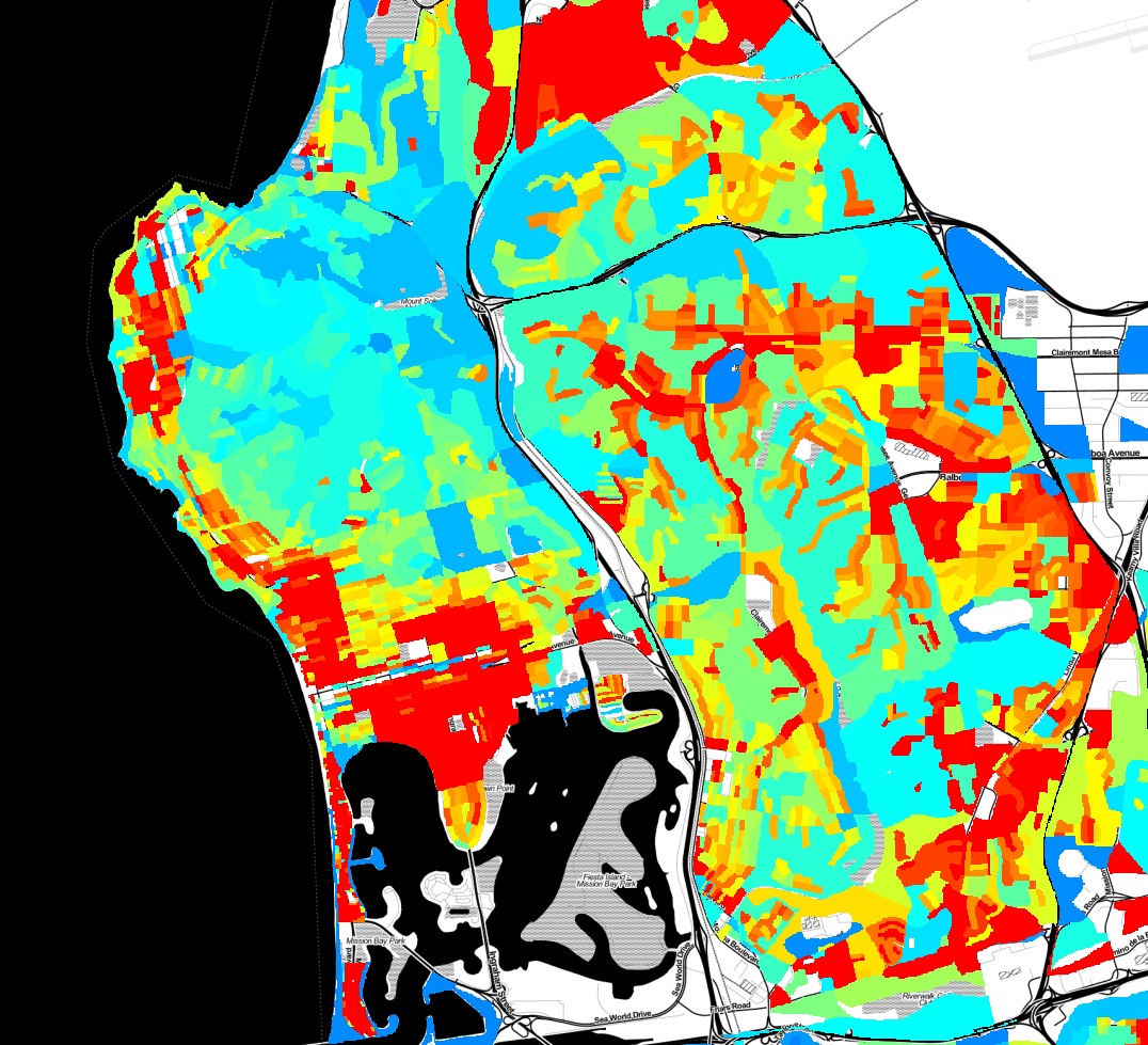
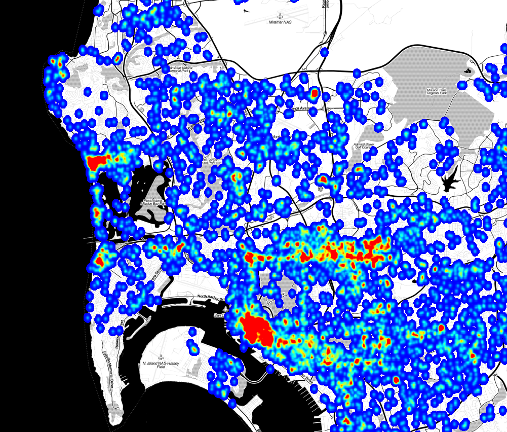
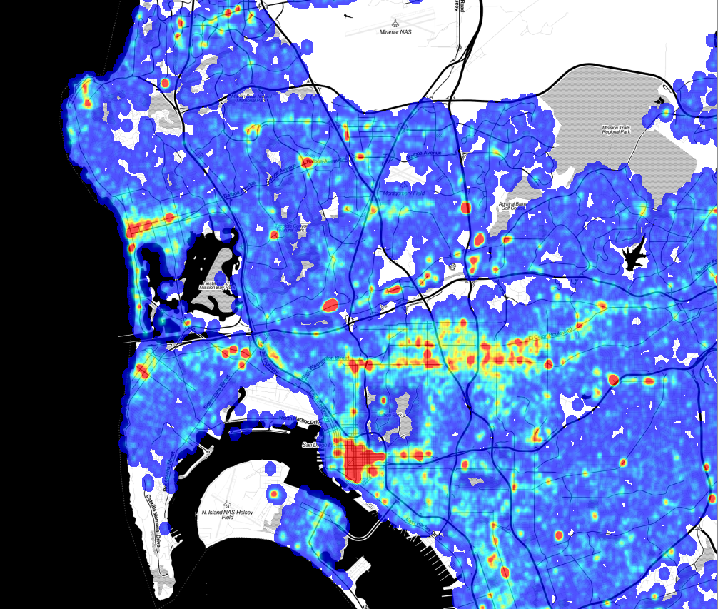
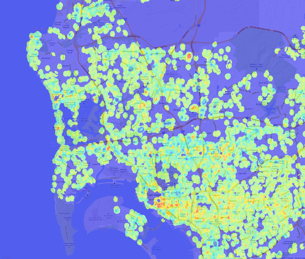
The Hot Spot tool calculates the Gi* statistic for each feature in a dataset. The resultant z-scores and p-values tell you where features with either high or low values cluster spatially. To have a statistically significant hot spot, a feature will have a high value and be surrounded by other features with high values as well. My animated maps illustrate 2 hot spots from 2007 to 2012. the most significant hot spot is located close to St. Vincent Paul homeless shelter ( Imperial Ave) on the South Eastern part of East Village. The second hot spot is located North of Gaslamp Quarter between Broadway And Market which most of the famous and popular bars are found. In addition to those map,and based on those hot spots, I did some statistical analysis to show the average of Drugs/ Alcohol violation monthly (Above/ Below Avg) and yearly. My study reveals that there is a slight increase within 2011 and 2012 in the average of Drugs/ Alcohol violations.
Continue Reading →

SANDAG Is Now Publishing Crime Data Weekly

SANDAG, through its public safety division ARJIS, is now publishing crime data to the web. This is a major advance in accessibility, since previously crime incidents were only available through a Public Records Act request, and usually involved a fee. The download file includes crime incidents for the last 180 days. The Library will be archiving these files occasionally, and adding them to our crime incident datasets. The files are updated weekly. Unlike the data we acquired previously, this release does not include the ’legend’ field, which is the high level category for the type of incident. As a result, we can’t incorporate these files into our previous releases without doing a lot of work to re-construct the ’legend’ field, so it may take a while before our datasets are getting updated.

Continue Reading →

Visualizing Traffic Accidents

We recently converted the SWITRS database of traffic collisions in California, extracting the records for San Diego County and creating a basic visualization in Tableau Public. Tableau Public is a fantastic data analysis tool, although it takes a bit of training to do complex things. Below is a simple visualization of the number of people killed and injured in San Diego county traffic collisions by day of week and hour of day, for the years 2002 to 2012, inclusive. The deaths line (orange) shows a familiar “bathtub” shape, with higher values on weekends and at night. The injured line is quite different. There are a lot of possibilities for this, including statistical effects due to the 100x difference in the number of injuries and deaths, or the qualitative differences between pedestrians at night during those of the day. For instance, it may be that injuries during the day are driven by travel patterns and reduced attentiveness in the afternoon, while fatalities are driven by alcohol consumption. Fortunately, there is enough information in the SWITRS dataset to test some of these hypothesis, but that will be the subject of another post.

Continue Reading →

Crime Data Update

We’ve released an update to the crime dataset today. This update is based on reprocessed data from SANDAG and includes some new fields.

San Diego Crime Incidents, Revision 3

This update is based on a new extract of the data we got recently from SANDAG. They didn’t tell me what had changed, just that they found some problems and re-ran the extract. If you want to compare the inputs, we have both the first revision and second revision of the SANDAG input data in the data repository. This release includes several new fields in the CSV and Shapefiles, including

Continue Reading →

Visualizing Infrastructure with Balloon Animals

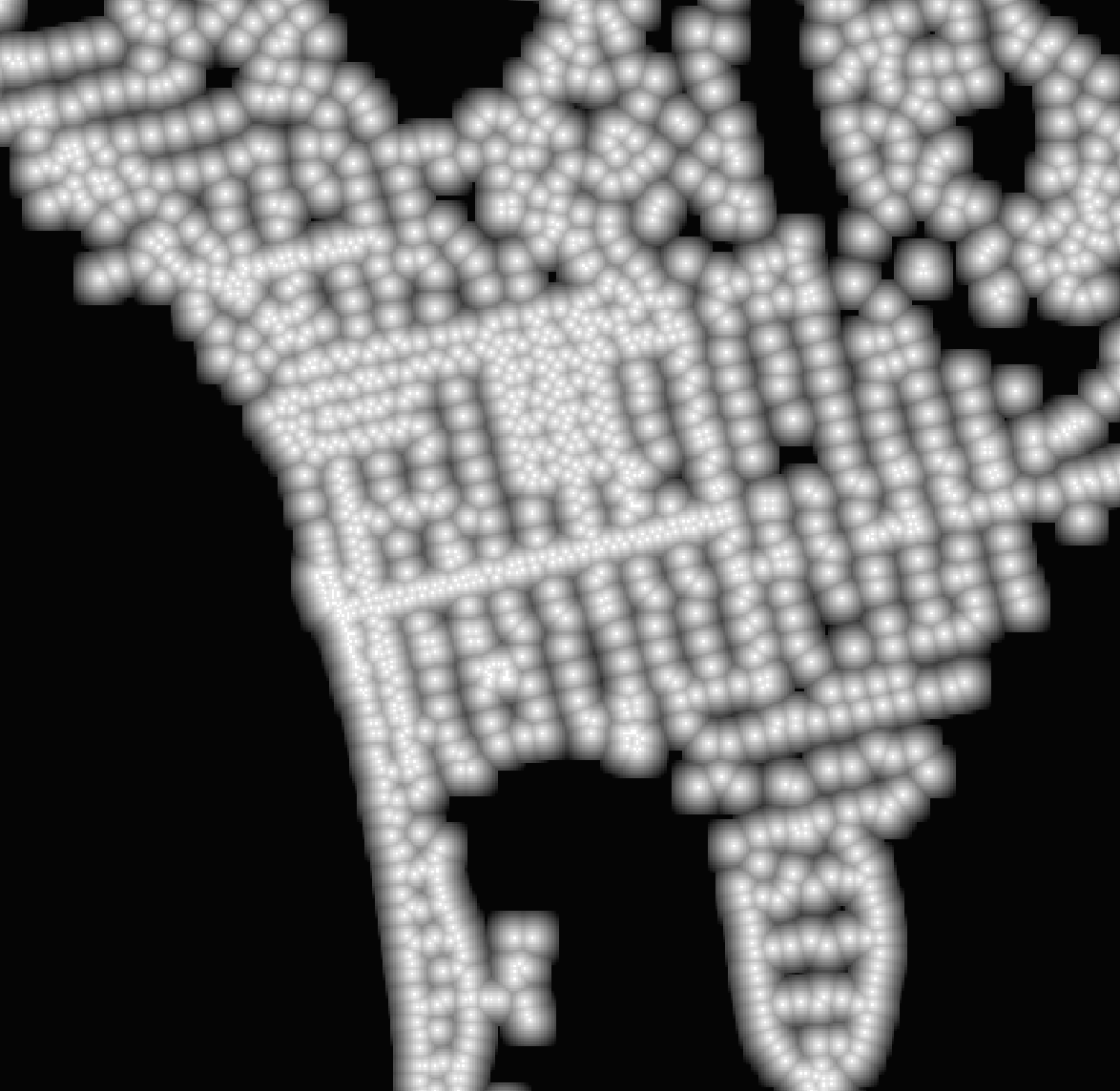
What if you got really creative with data visualization and represented the street lights of La Jolla and Pacific Beach with the balloons that are used to make animals? It might like like this: An image of a dataset showing the distance, in centimeters, to the nearest street lamp. An image of a dataset showing the distance, in centimeters, to the nearest street lamp.   This image is actually from a dataset I’ve created showing, for every 10m^2 area of the City of San Diego, how far the point in the middle of the area is from a street lamp. The image is colored so white is 0m and black is about 141m from the lamp. We’ll be using this data in our Crime Analysis Project to explore the connect between street lamps and crime.

Continue Reading →

Six Years of Crime Data

Today we are releasing the processed version of six years of San Diego County crime data. We received this data last month from SANDAG, and have augmented the source data with city and and neighborhood codes. The data is released as both CSV and ESRI Shape files with one file per year. To download the data, visit our data repository. Be sure to read the documentation by expanding the pull-down bar at the top of the page. The improvements of this dataset over the original SANDAG data release include:

Continue Reading →

Crime at Street Segments

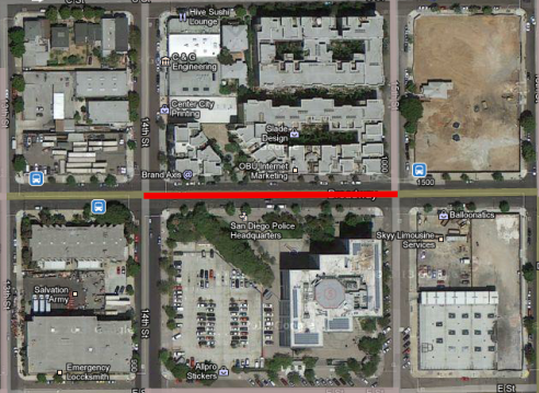
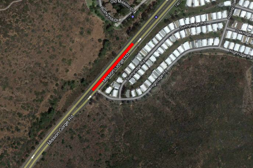
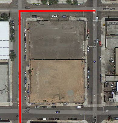
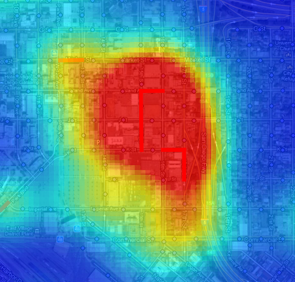
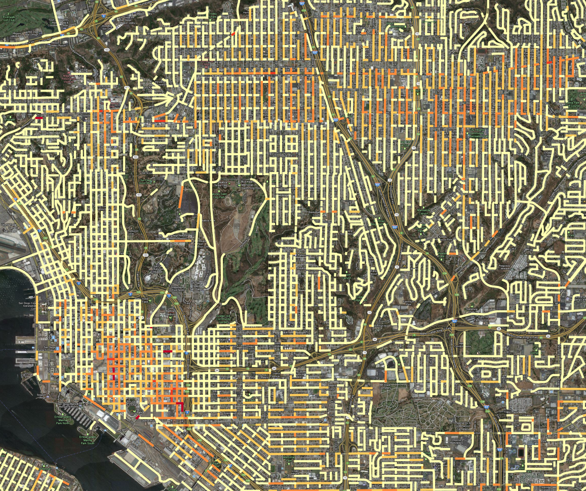
A few weeks ago, we received crime incident data from SANDAG for the years from 2007 to March of 2013. The data has the location of the crime listed as a “hundred block,” so a crime at 1435 Main street would be listed at 1400 Main. Since we don’t know where the crime occurred on the block - we don’t know the exact address - it makes sense to attribute the crime to the whole block. I just finished an initial pass at geocoding crimes to street segments, using the All_Roads file from SANGIS and lot of custom Python code. Here are the results: All crime incidents for 2007 to 2013, colored according to linear density on the street segment. All crime incidents for 2007 to 2013, colored according to linear density on the street segment. In this map, all of the crime incidents for the 6 year period are counted, grouped by the block where the crime occurred. Then, the counts are divided by the length of the street segment and the time period, so the final value is Crime per year per kilometer. Then, the range of values is broken into 5 groups, using the Jenks natural breaks. ( Using head/tail breaks would require more programming ) I tweaked the breaks manually to put more segments into the top category. This presentation has an advantage over the previous maps we’d created, using Kernel Density Estimation to produce heatmaps: it is easier to see where high-crime blocks are. For instance, lets look at the red block east of downtown, due south of Balboa park. A crack house, perhaps? Police Station PM Nope, it is the Police station. It is very common for crimes to have their address set to the police station if it isn’t clear what an appropriate address would be, such as for a car chase or someone caught in a canyon, like in this hotspot in Mission Gorge: Mission Gorge   It isn’t likely that the particular segment of road gets a lot of crimes, and the criminals probably don’t live in the mobile home park. That segment of road probably contains the address number that is used for crime committed in Mission Gorge, it maybe it is where the cops like to park to patrol the canyon. Here is a real hotspot, an empty lot that seems to be popular for drug use: Downtown Drug Lot Compare this to the heatmap view, zoomed out to show the contour of the hotspot: Drug Area Heatmap The heatmap works better at small scales, because you can quickly assess an entire region. At large scales, the street segment view can help isolate what a likely cause of the problem is, which can obscured by the large regions of the heatmap hotspots. The heat map also encourages a subtle psychological bias: the larger areas seem more significant, because our brains place a lot of emphasis on size. But in the segment map, the segments are viewed discretely, as qualities, not extents. So, it is easier to pay attention to unusual high intensity blocks which pop up because they are bright red, but which in the heatmap get ignored because they are small. We’re not quite ready to publish the processed crime data, but should have it released, along with both kinds of maps, in the next week.

Continue Reading →

Population Density Maps

Here is some eye candy, a population density map of Pacific Beach and surrounding neighborhoods.

population-density-map

This map was created with a lot of Python code, using the 2010 census shapefiles for census blocks, setting a value for each block as the population of the block divided by the area of the block, and rasterizing all of the blocks to an image. Red indicates areas of higher population density. You can clearly pick out the areas in Pacific Beach that are zoned for apartments vs single family homes, the UTC high-rise apartment area, and many other variations in land use.

Continue Reading →

TGIF Chula Vista, It's Crime Minimum Day

Our resident data slinger sent me an initial analysis of time series data for specific crime hot spots in San Diego, and the results are interesting. Rather than look at the whole of the region at once, we’ve identified specific high intensity areas, and are doing time-series analysis for them independently. The major areas are: North Park, Chula Vista, Gaslamp and Pacific Beach. Since each of these areas is very different, they have different crime profiles, so we’re analyzing them separately. Here is the map for the Chula Vista analysis area:

Continue Reading →

Property vs Violent Crime

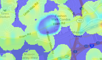
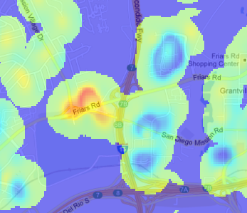
As part of our upcoming Crime Mapping project, we’ve started producing maps of San Diego area cime incidents, and have made a few interesting discoveries that we’d like to share. While these aren’t ground-breaking insights, the results do confirm intuition and offer some small surprises. A few months ago we received and processed the SpotCrime.com free database, a database of crime incidents from across the country for the years 2007 to 2011. This data was scraped from many different police department websites, although the San Diego data was all scraped from ARJIS ( part of SanDAG ) before SANDAG changed the map software, eliminating the possibility of free acess. This database is a wonderful resource, and even though the data does not have an official pedigree, there are enough datapoints to do some useful work. SpotCrime is providing an incredible benefit by offering this data. Thanks! Our first stage of analysis involves creating heatmaps from the incidents. To create these maps, we quantized the incidents into bins 1/5000 of a degree square, about 19m. Since the records are typically reported with a “hundred block address” – “1300 Wilbur Ave” instead of “1324 Wilbur Ave” – we added a bit of randomness to the points. While this isn’t exactly correct, as it randomly moves the incident by up to 100m, it does space the points out in a more natural way. Then, for each incident, we spread out the crime point ( with a 2-D Gaussian, fwhm = 57m) to smooth out the image. The spreading also simulates both the extended “influence” of a crime, and the fact that a crime at one point means it is more probable that a crime will occur at nearby points. Violent crimes are separated from from the property crimes with a separate map for each. Here is the violent crime map: ( Click to Enlarge) Violent Crime Incidents, 2007 - 2011. Data from SpotCrime.com Violent Crime Incidents, 2007 - 2011. Data from SpotCrime.com The red spots are the areas of the highest number of crimes, and almost all of them are entertainment districts. Violent crime tends to occur at night, where there are a lot of people, and where people are drinking, and an entertainment district has all three conditions. Here is the map of the property crime incidents. This has more complete coverage because there are a lot more property crime incidents than violent crime incidents. Property Crime Incidents, 2007 to 2011. Data from SportCrime.com Property Crime Incidents, 2007 to 2011. Data from SportCrime.com There are a lot of similarities in where the crimes occur, but the property crimes are more diffuse, and there are many small-scale differences. To find the differences between the two, we can subtract the two maps. In this image, blue indicates areas where property crimes dominate, green is neutral, and red is an area where violent crimes dominate: Property / Violent crime DIfference Violent crime density minus property crime density. Note that in this map, green does not mean “good,” it means that the difference in the density of violent crime and property crime is nearly equal. The green areas can have very high violent crime rates; being green just means they also have high property crime rates. This map gets really interesting when you zoom in to look at specific spots. Closer examination doesn’t reveal a lot of new discoveries, but it does confirm intuition about where we should find property and violent crimes. Fashion Valley MallThis high-property crime area is Fashion Valley Mall. It seems sensible that the mall would be a target for theft, but the upscale shoppers don’t often get into altercations. Mission Valley mall has a similar emphasis on property crimes.
Qualcomm StadiumQualcomm stadium, in red, is a hot spot for rowdy sports crowds, but the apartments along the golf course, while actually having a higher than average violent crime rate, see relatively more property crime.
(There is an interesting error in the difference map. The values for each map are scaled so that the range of ±4σ in the original output maps to (0,1] in the final output, so high outliers all have the value of exactly 1. This means that for an area with both high property and violent crime, the difference is exactly 0, which is the no data value. This is why Garnet street in Pacific Beach and the Gaslamp district have areas of no data in the difference map. ) A map like this has a lot of interesting stories to tell, even though the analysis is not very rigorous. We started with data that we can’t vouch for, added randomness, created a map with a lot of arbitrary choices, and ended up with useful insights. The entire process emphasizes that even when data and analysis are not of sufficient quality to make statistical inferences, we can still extract useful knowledge.
Continue Reading →